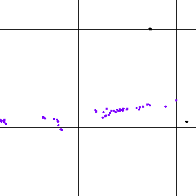
This is an example of an attempt to simultaneously invert for model parameters and hypocentral parameters of the sources from the given arrival time data provided by James Rutledge. This set of data files is denoted by "CV" according to the site name "Cotton Valley".
'cv-arr.dat', 'cv-stn.dat' and 'cv-list.dat' are the original data files by James Rutledge. Their original file names were 'leo_75events_arrivals.dat', 'stn_list_loc.dat' and 'leo_top75_event_list.dat'.
'cv-arr.dat'
contains the P-wave and S-wave arrival
times of 75 events recorded at 13 receivers.
For each event there are 14 lines.
The 1st line is the event name, next 13 lines are the picks and
hodogram azimuths to source, if reliably determined:
station, Ptime, Stime, az
A value of zero means no pick or no azimuth determined.
Time is in seconds from the start of record, azimuth in degrees clockwise
from north.
'cv-stn.dat' contains
the names and coordinates of 13 receivers:
stn_name, N, E, Z
Coordinates are in feet. The receivers are located in 2 vertical wells.
'cv-list.dat' is the list of the names of 75 events.
'cv-arr.for' is a simple program reading file 'cv-arr.dat', separating P-wave and S-wave arrival times and writing them into files 'cv-arrp.dat' and 'cv-arrs.dat' with the P-wave and S-wave arrival times reformatted for the SW3D software.
'cv-rec.dat' are the receiver positions from file 'cv-stn.dat', reformatted for the SW3D software.
A questionable manual location using program 'cv-src.for' was used to estimate an initial homogeneous model and initial source positions for linearized simultaneous inversion. After first tests, the vP/vS ratio was fixed to SQRT(3), and a range of trial vP velocities was estimated. For a given vP velocity, hypocentres were roughly estimated by means of program 'cv-src.for' and arrival time residuals were calculated. The homogeneous model and hypocentres with the smallest residuals were selected. The velocities are vP=18034 and vS=10412. File 'cv-src.dat' contains the roughly estimated hypocentral coordinates and times.
Two-point ray tracing in a model temporarily named 'cv-mod.out' for the file with coordinates of sources temporarily named 'cv-src.out' is performed by the history file 'cv-crt.h'. The receivers for two-point ray tracing are projected onto the vertical reference plane approximately given by the 2 vertical wells. 'cv-crt.dat', 'cv-cod.dat', 'cv-rpa.dat' and 'cv-writ.dat' are the data for ray tracing by program 'crt.for'. 'cv-crtp.dat' and 'cv-crts.dat' are the lists of results of ray tracing for P and S waves used in the inversion.
A single iteration of simultaneous inversion for a velocity model and hypocentral coordinates is performed by the history file 'cv-inv1.h'. It uses the results of ray tracing in the initial model of the iteration. The file with initial source coordinates is temporarily named 'cv-src.out'. The initial model is temporarily named 'cv-mod.out', and coincides with the template model describing the parametrization of the final model of the iteration. The final model of the iteration is also named 'cv-mod.out' and thus overwrites the initial model. The file with final source coordinates resulting from the iteration is temporarily named 'cv-srcn.out'.
'cv-srf.dat' is the auxiliary model file specifying the vertical reference plane. It is only used during inversion to check the distances of hypocentres from the reference plane. 'cv-sob.dat' is another data file used in the inversion. It specifies the Sobolev norm minimizing the horizontal velocity gradient to find a 3-D model close to 1-D.
The whole simultaneous inversion for a velocity model and hypocentral coordinates is performed by the history file 'cv-inv.h' repeatedly executing history files 'cv-crt.h' and 'cv-inv1.h'. The inversion may be performed with various initial models and with various parametrizations of final models (homogeneous, 1-D, 3-D).
'cv-mod0.dat' and 'cv-src0.dat' are files with the initial homogeneous velocity model and with corresponding initial source coordinates. File 'cv-src0.dat' differs from file 'cv-src.dat' by one source slightly shifted away from the reference plane only.
'cv-mod1.dat' and 'cv-src1.dat' are files with the homogeneous velocity model and with corresponding source coordinates resulting from 3 iterations starting with model 'cv-mod0.dat' and sources 'cv-src0.dat'. Homogeneous velocity model 'cv-mod1.dat' has been converted into 1-D parametrization.
'cv-mod2.dat' and 'cv-src2.dat' are files with the 1-D velocity model and with corresponding source coordinates resulting from 3 iterations starting with model 'cv-mod1.dat' and sources 'cv-src1.dat'. 1-D velocity model 'cv-mod2.dat' has been converted into 3-D parametrization.
'cv-mod3.dat' and 'cv-src3.dat' are files with the 3-D velocity model and with corresponding source coordinates resulting from 2 iterations starting with model 'cv-mod2.dat' and sources 'cv-src2.dat'.
'cv-mod04.dat' is just the initial homogeneous velocity model 'cv-mod0.dat' converted into 3-D parametrization.
'cv-mod4.dat' and 'cv-src4.dat' are files with the 3-D velocity model and with corresponding source coordinates resulting from 9 iterations starting with model 'cv-mod04.dat' and sources 'cv-src0.dat'.
PostScript files
'cv-src.ps',
'cv-src0.ps',
'cv-src1.ps',
'cv-src2.ps',
'cv-src3.ps' and
'cv-src4.ps'
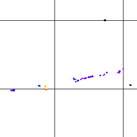
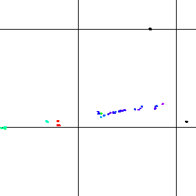
are the plots of horizontal positions of source
points from corresponding data files '*.dat'.
Hypocentral positions in 'cv-src.ps' are colour-coded according
to the P-wave velocity, i.e., all hypocentres have equal colour.
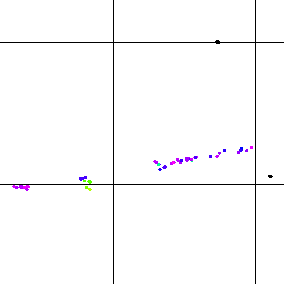
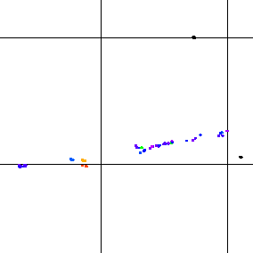
Hypocentral positions in 'cv-src1.ps', 'cv-src2.ps', 'cv-src3.ps'
and 'cv-src4.ps' are colour-coded according to the hypocentral
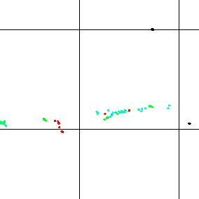
depth (9000 M, 9070 B, 9140 C, 9210 G, 9280 Y, 9350 R).

|
| Fig. 1: Hypocentral positions calculated analytically as an initial estimate for a homogeneous model. |
|
| Fig. 2: Hypocentral positions calculated analytically as an initial estimate for a homogeneous model, one source is slightly shifted away from the reference plane. The positions are colour-coded according to the hypocentral depth (9000 Magenta, 9070 Blue, 9140 Cyan, 9210 Green, 9280 Yellow, 9350 Red). |
|
| Fig. 3: Hypocentral positions calculated after 3 iterations in a homogeneous model starting from the analytically estimated homogeneous model. |
|
| Fig. 4: Hypocentral positions calculated after 3 iterations in a 1-D model starting from the homogeneous model. |
|
| Fig. 5: Hypocentral positions calculated after 2 iterations in a 3-D model starting from the 1-D model. |
|
| Fig. 6: Hypocentral positions calculated after 9 iterations in a 3-D model starting from the analytically estimated homogeneous model. |
It is obvious from the above mentioned numerical experiments that the arrival times are not sufficient to simultaneously estimate both the velocity model and hypocentral coordinates. The arrival times would be sufficient to approximately determine hypocentral coordinates in a given velocity model. On the other hand, the simultaneous inversion can simply adjust the velocity model to given hypocentral coordinates.
The arrival times combined with velocities from well logs may be used to estimate a 1-D mean velocity model. The velocities from well logs may then be used to estimate the correlation function describing the inaccuracy of the 1-D mean velocity model. The location may then be performed in the 1-D mean velocity model. The inaccuracy of the location may then be estimated using the correlation function.